From a patient to a dose — and every equation in between.
A walkthrough of the real calculator, followed by a complete account of the
mathematics and the population models it uses, each tied to the paper it came from. Every screenshot is a
synthetic demo patient, never a real one. This is orientation, not clinical advice — the tool is decision
support, and every number it produces still wants a clinician's judgement.
Five words first
AUC24
The total drug exposure over a day — the area under the concentration-time curve. Vancomycin's
efficacy and its kidney toxicity both track exposure rather than any single concentration, which is
why the 2020 guideline made this the target and retired trough-only dosing.
Trough
The lowest concentration, just before the next dose. Still worth measuring — it is what an assay
actually returns — but it is no longer a target. Many different exposure profiles can produce
an identical trough.
Clearance (CL)
Volume of blood cleared of drug per hour. It sets the exposure: at steady state, AUC24 = daily dose ÷ CL.
Volume of distribution (V)
The apparent volume the drug spreads into. It sets how high the peak goes and how fast the level swings between doses.
Bayesian / MAP
A method that starts from what is typical for a population, then bends towards this patient as their
own measured levels arrive. With one level it moves partway; with more, further. It never ignores the
data, and never fully abandons the prior.
The walkthrough
01
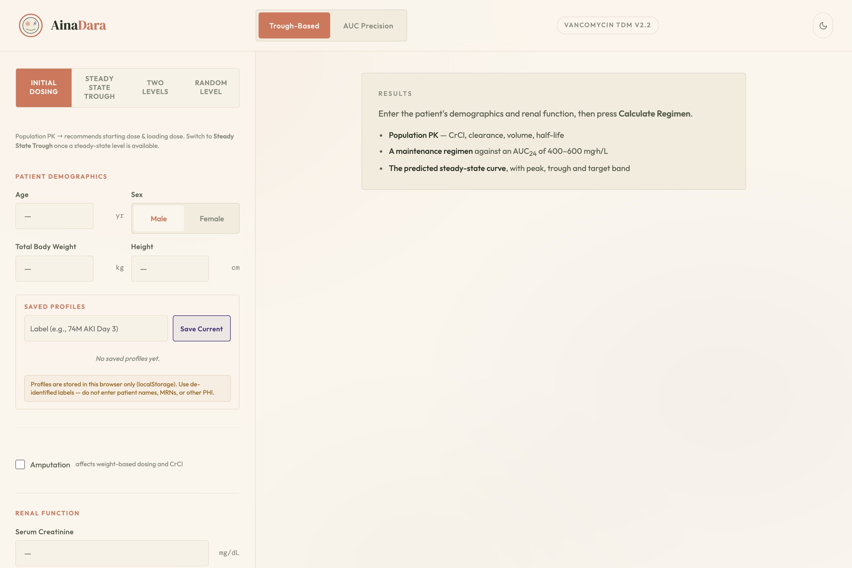
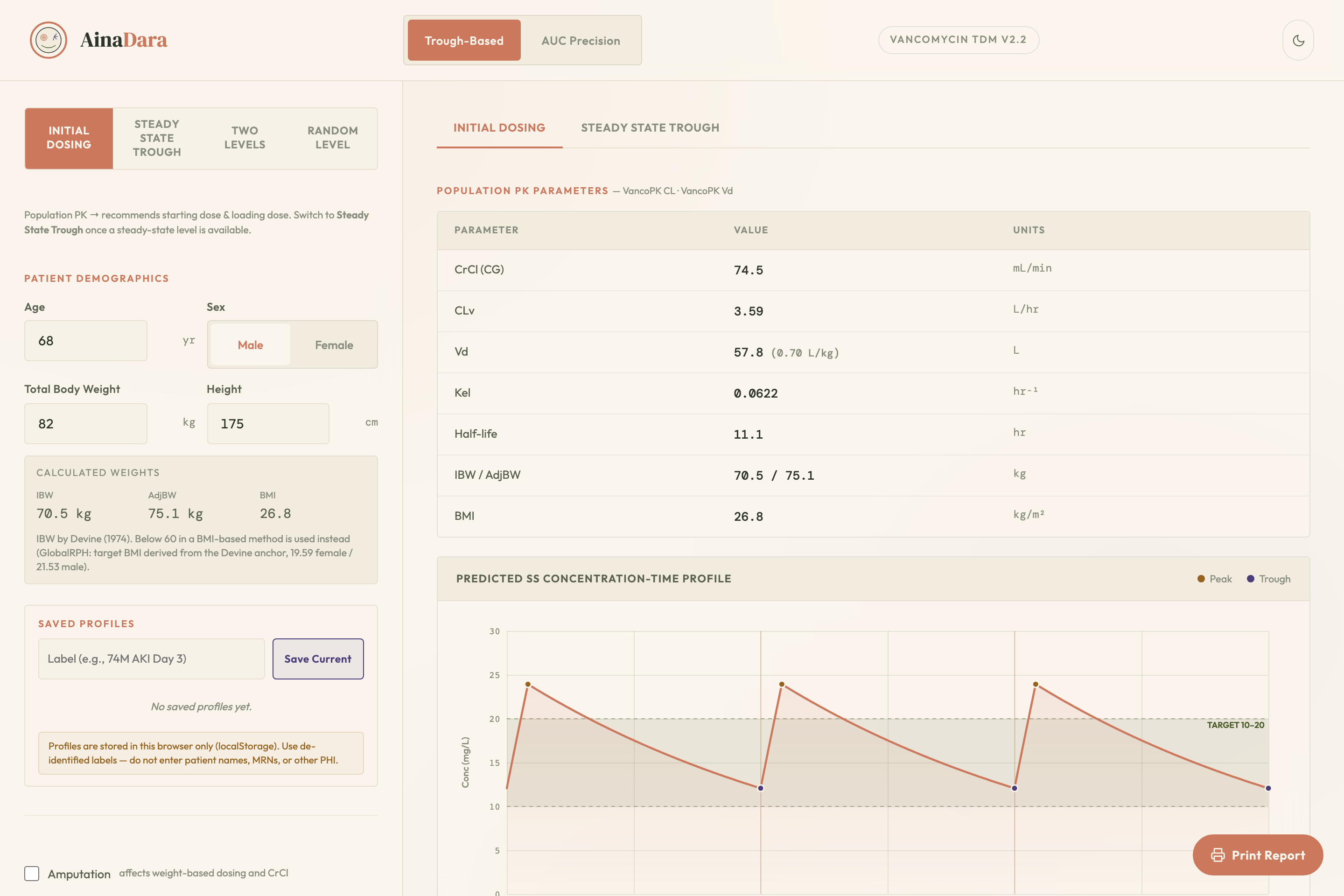
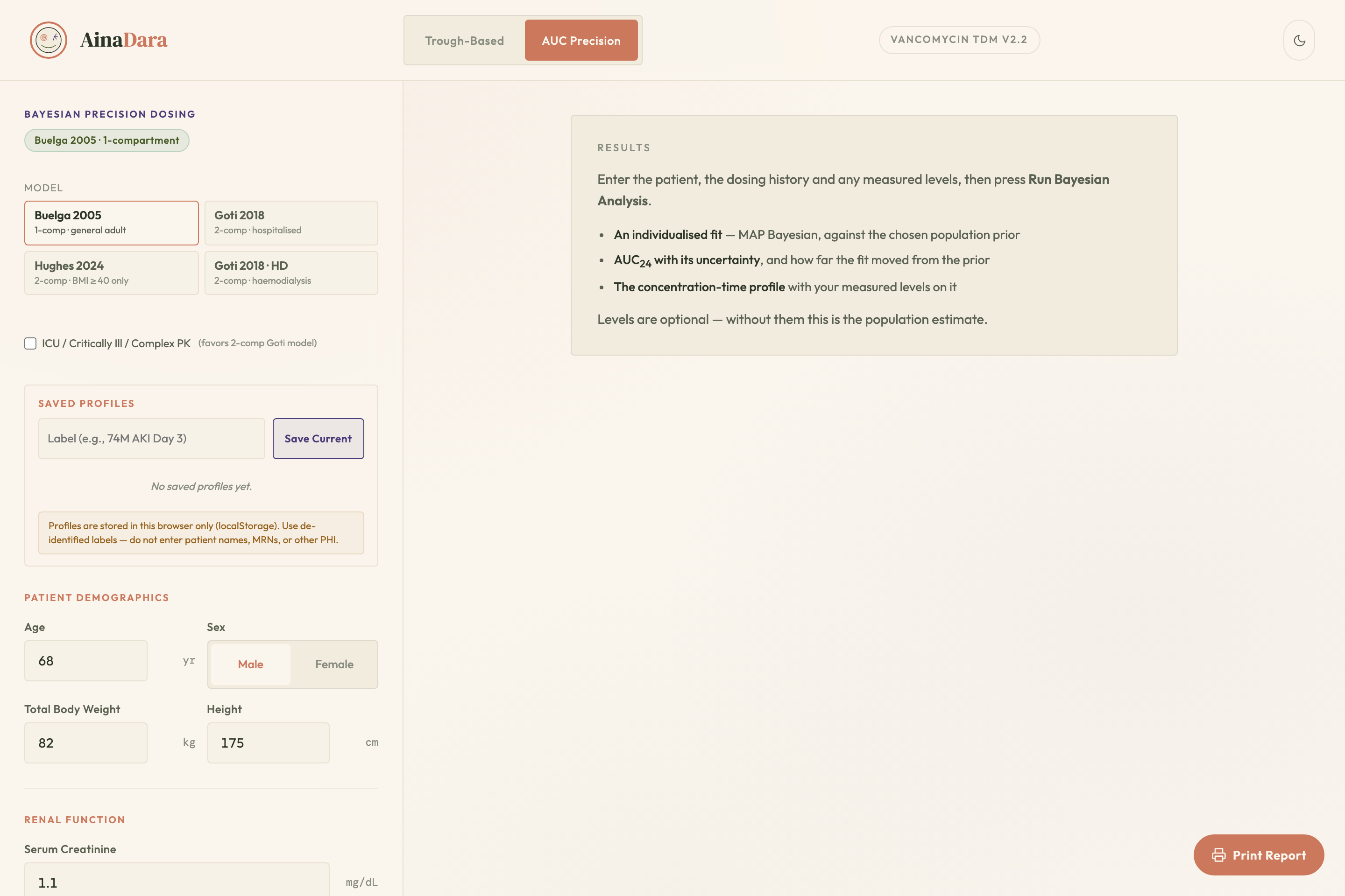
Open the tool
Inputs on the left, answers on the right. Two modules across the top:
Trough-Based for deterministic dosing, and AUC Precision
for Bayesian fitting once you have levels. Saved profiles work in both — save from either
and loading fills both, so a patient is entered once. Nothing leaves the browser: there is
no server and no network call.
02
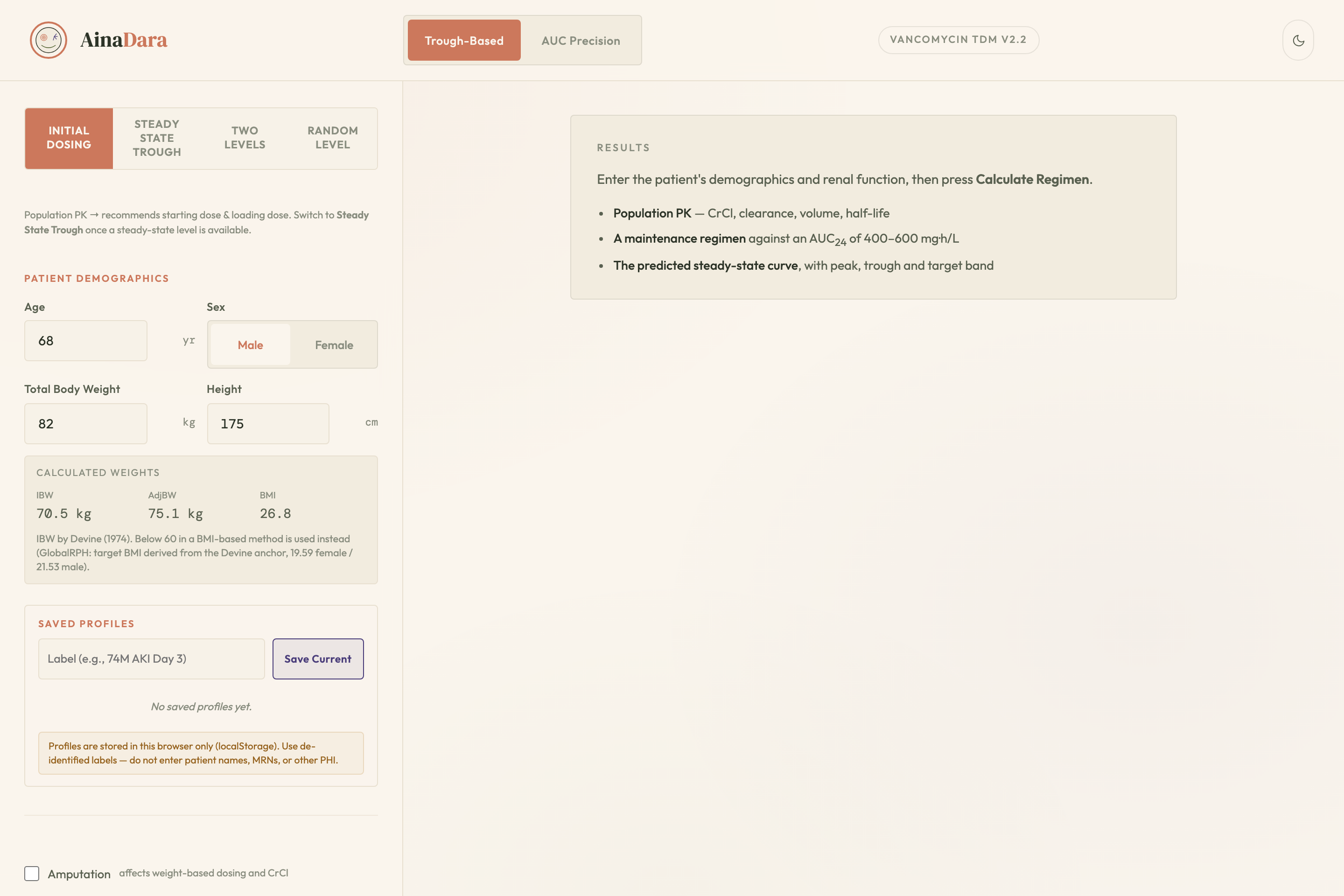
Describe the patient
Age, sex, height, weight and creatinine. The tool derives ideal and adjusted body weight and shows
the creatinine clearance it will use, naming the weight basis so you can see which one it chose.
The creatinine is used exactly as entered — it is never rounded up. If cystatin C
is available, entering it surfaces a creatinine/cystatin discordance check, which is the honest
answer to the low-muscle-mass problem that rounding was invented to paper over.
03
Read a starting dose
A starting regimen from population pharmacokinetics before any level exists. Choose the clearance
and volume models on the right; the panel underneath states the provenance of whichever you pick.
Expect roughly ±35% uncertainty on exposure at this stage — that is what "no levels yet" means,
and the tool says so rather than implying precision it does not have.
04
Enter the actual course
Enter what the patient actually received — every dose, its infusion duration, and the real
administration time — then the measured level and when it was drawn. Times matter more than people
expect: the fit is only as good as the timestamps. Rows that are started but incomplete are
reported rather than silently dropped.
05
Fit this patient
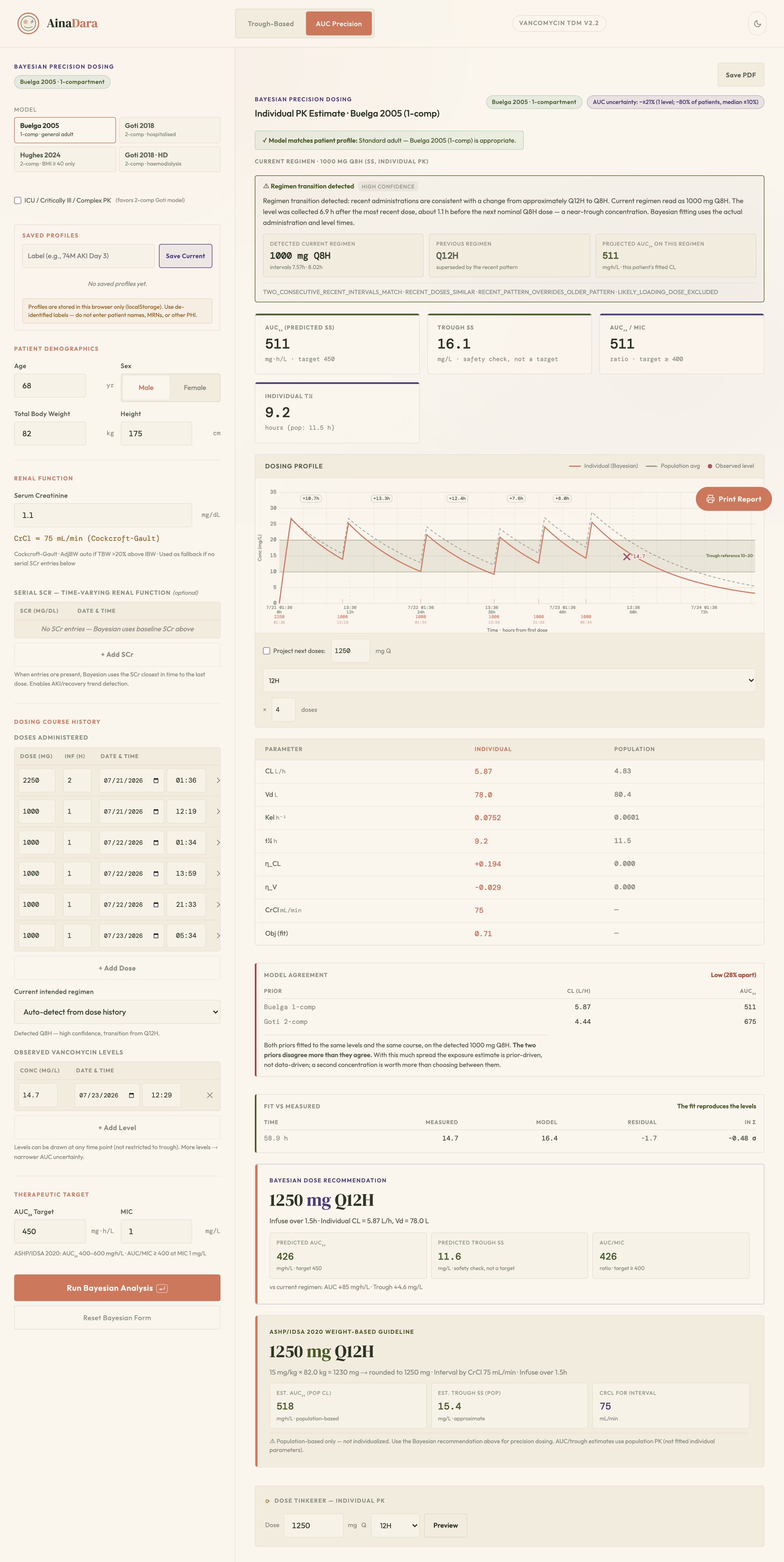
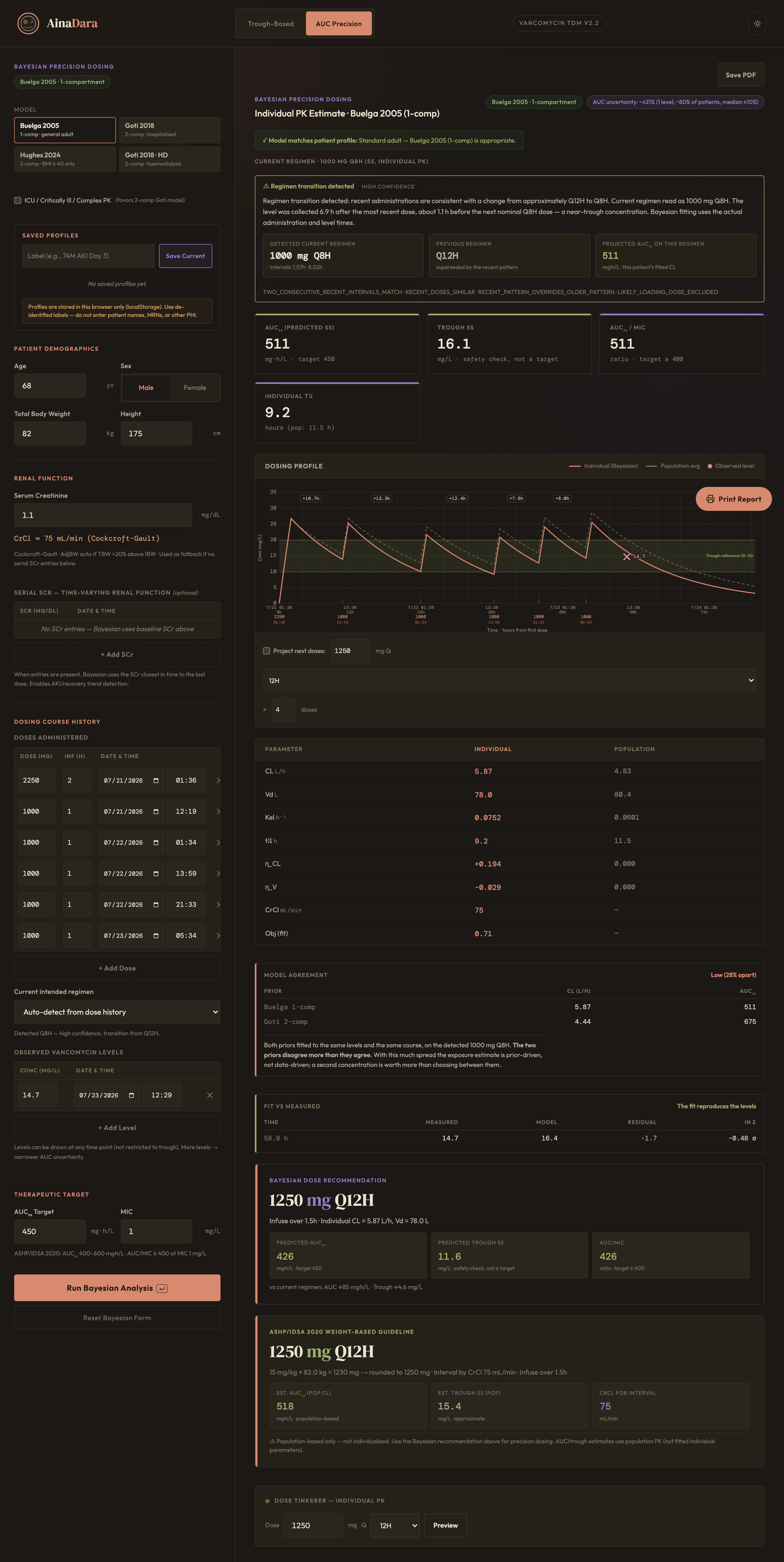
The fit. Read it top-down: the regimen the tool believes the patient is on (with its confidence,
and whether it detected a change of interval), then the fitted clearance and volume beside the
population values, then the recommendation. The banner in this example reports a genuine
q12h → q8h transition — detected from the two most recent intervals rather than from whichever
interval appeared most often. If you know the intended order, set it in
Current intended regimen; that steers the projection and never alters the data the fit
consumes.
06
Read the profile
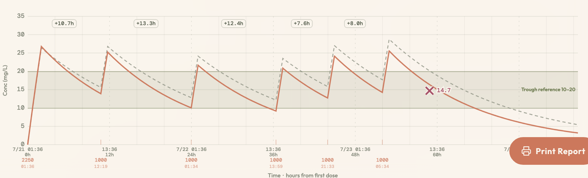
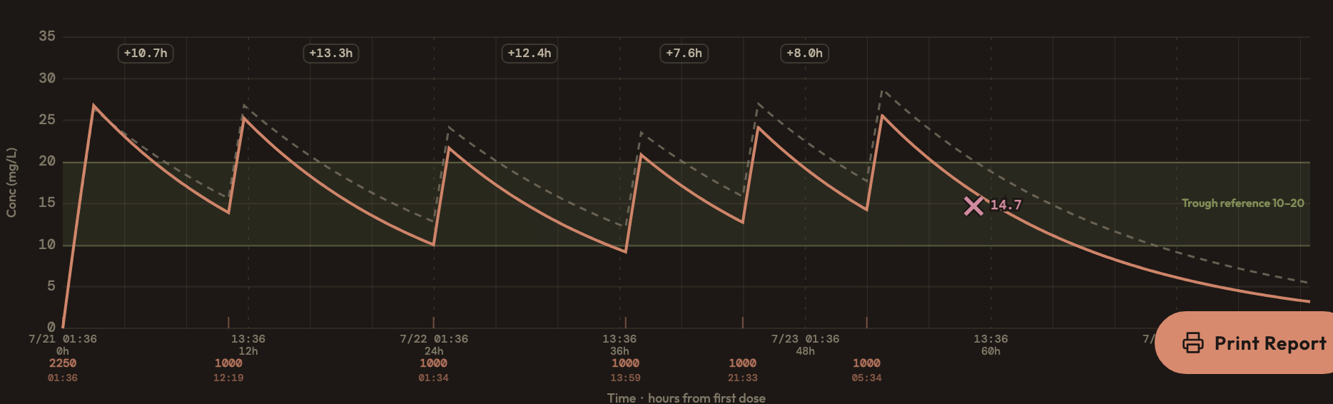
The solid line is this patient; the dashed line is what the population model predicted before their
levels were known. The gap between them is what the measurement bought you. Points are measured
levels, vertical marks are doses with the interval between them annotated, and the shaded band is
a trough reference — not a target. Hover anywhere on the curve to read the fitted concentration at
that instant, the clock time, and how long it has been since the last dose.
Every time is a date and a time
Doses and levels are entered as full timestamps everywhere in the tool — never a bare clock
reading. This is not tidiness; it is the difference between a correct answer and a confidently
wrong one.
Two-level sampling routinely spans midnight. A dose at 10:22 and a level at 10:38 the next
morning are 24.3 hours apart, but from clock readings alone that is
indistinguishable from 16 minutes. Earlier versions of this tool resolved the ambiguity by
assuming the same day and adding 24 hours only when the result went negative, which folds
every interval into the range 0–24 h.
That has two consequences, and the quieter one is the dangerous one. When the second level
wraps below the first, the solver refuses and says so. But when both levels
fall on a later day they shift by the same 24 hours, the log-linear slope between them is
unchanged, and the elimination rate still comes out right — while the back-extrapolation to
the peak, which uses the absolute time, is a full day early. Volume of distribution then comes
out several-fold wrong with nothing on screen to suggest it. A dose at 08:00 with levels at
12:00 and 18:00 the next day gave a Vd of 75 L where the truth was 13 L.
Each field now carries its own date, and the tool prints the elapsed interval back to you —
1d 0.3h (total 24.3h) after dose start — so you can confirm it
read the timestamps the way you meant them before you trust anything downstream. A level dated
before its dose is reported as an error rather than silently absorbed.
Reading the graph
The plot exists so you can estimate a concentration at a time point. Its axes are built for
that, and a few of its choices are deliberate enough to be worth stating.
The time axis is your interval, not a constant
Ticks are placed at half the dosing interval, so there are always seven of them and
every dose boundary falls on one — at Q6H they land on 0, 3, 6, 9, 12, 15 and
18 h; at Q48H on 0, 24, 48 and so on. You can therefore read the trough directly off a
gridline rather than interpolating toward it. The vertical terracotta rules mark where each
dose is given.
This replaced a fixed 8-hour tick that aligned with no dose boundary at Q6H, Q12H, Q18H, Q24H,
Q36H or Q48H, and drew nineteen overlapping labels at Q48H.
The concentration axis contains everything drawn on it
The vertical range is chosen to include the curve, the target band, and any measured
level — not just the curve. That matters for a low-dose regimen in a fast clearer: if the axis
followed the curve alone, a 10–20 mg/L band would be painted off the top of a plot whose peak
was 8 mg/L, and the band would read as "everything above 10 is on target." Gridlines are placed
on round values at a roughly constant density whatever the scale.
The shaded band is your target, and it is a reference
The band is drawn from the trough range you entered, and labelled with those bounds —
it is not a fixed 10–20. It is shaded for orientation only: the 2020 guideline withdrew trough
as a target (Rec 3, A-II) and AUC24 governs. It stays on the chart
because a trough is still the value a level actually measures.
What each mark means
Mark
Meaning
Rose ×, with a value
A measured level. The only real number on the chart; everything else is a model. Drawn above the curves so nothing hides it.
Solid terracotta line
This patient's fitted concentration-time curve.
Dashed neutral line
What the population model predicted before the levels were known. The gap between the two is what the measurement bought you.
Solid purple line
Projection under doses that have not been given yet.
Amber and purple dots
Predicted peak (end of infusion) and trough (end of interval).
Shaded band
Your trough reference range, labelled with its bounds.
Markers are drawn on the curve, not near it — the curve is sampled at the end of infusion and
at each interval boundary specifically so the peak dot sits on the line rather than above the
corner the polyline would otherwise cut. If a marker ever appears off the curve, that is a bug,
not rounding.
One place the marker genuinely cannot lie on the curve
In Random Level mode the level is fitted against single-dose decay while the
chart draws a steady-state profile. These are different models, so the plotted point and the
drawn curve will not coincide, and that is expected rather than an error. Read the fitted
parameters, not the visual fit.
Choosing the interval — and why the tool will not do it for you
The tool computes exposure. It does not choose your dosing interval, and the reason is
arithmetic rather than modesty.
At steady state the area under the curve over 24 hours is simply the total daily dose divided
by clearance:
AUC24 = dose x (24/tau) / CL = total daily dose / CL
There is no interval term in it. 500 mg every 12 hours and 1000 mg every 24 hours
deliver exactly the same exposure, and so does 2000 mg every 48 hours. Any rule that
ranks regimens on how close their AUC24 sits to a target is therefore blind to the interval by
construction; whichever interval happens to reach a daily dose nearest the target wins, and
with doses rounded to 250 mg that is decided by rounding rather than by pharmacology. The
rounding is not even-handed either — one 250 mg step moves AUC24 six times less at Q48H than
at Q8H, so a long interval can always land closer.
Rather than hide that behind a tuned preference score, the tool shows the whole picture. The
exposure matrix lays out every dose against every interval, shades each cell
against the 400–600 mg·h/L band, strikes through anything that breaches a hard safety limit,
outlines the recommended cell, and lets you click any other one to see its full profile. The
AUC values repeat down the diagonals, which is the point: those regimens are exposure-
equivalent.
What does change with the interval is the shape — peak and trough. Those are yours to weigh
against renal trajectory, how long you expect the regimen to stand, infusion-related
tolerability and practicality on the ward. The tool gives you the numbers for each; the
judgement is not something it can derive from an AUC target.
The single recommendation is still shown, because a starting point is useful. Treat it as one
admissible cell among several rather than as a ranking the model has earned.
The mathematics
Everything below is implemented in the shipped file and covered by an automated suite that runs the real
engine — 101 unit and regression tests, 21 simulation checks, and 40 regimen-detection cases. Fifteen of
those run the actual chart renderers and assert on what they draw.
Body size and renal function
Ideal body weight. At or above 60 in (152.4 cm), Devine (1974):
IBW = 50 (male) or 45.5 (female) + 2.3 x (height_in − 60)
Below 60 in, Devine extrapolates downwards and understates IBW, so the GlobalRPH BMI method is used
instead — with the target BMI derived from the Devine anchor rather than chosen:
IBW = (50 ÷ 1.524²) x height_m²  = 21.53 x height_m²   (male)
IBW = (45.5 ÷ 1.524²) x height_m²  = 19.59 x height_m²   (female)
Deriving the target from the anchor is what makes the two methods meet: IBW is continuous and monotonic
across 152.4 cm. Substituting round numbers such as 21.5 / 22.0 — a different method entirely
(Tokunaga 1991) — breaks the join and makes a 152.3 cm woman weigh more than one at 152.5 cm.
Adjusted body weight — AdjBW = IBW + 0.4 x (TBW − IBW), used for creatinine clearance when total weight exceeds IBW by more than 20%. Where actual weight is below the selected basis, actual weight wins.
Creatinine clearance — Cockcroft-Gault, on the measured creatinine:
CrCl = ((140 − age) x weight) ÷ (72 x SCr) x 0.85 if female
No rounding of low creatinine. Rounding up in the elderly under-doses measurably: in 56 patients aged
≥65 with baseline SCr <1, rounded creatinine missed measured troughs by 8.84 mg/L against 4.54 mg/L
for the actual value, and 92.9% came out subtherapeutic (Drugs R&D 2017;17:463-70). The one exception
is internal to the Goti model, which was estimated on truncated creatinine and so must be fed
the same transformation — that never touches the creatinine clearance shown on screen.
One-compartment infusion, at steady state
With R0 = dose ÷ t_inf, ke = CL ÷ V, interval tau:
Dropping that second term is a real and easy mistake — it agrees with the correct form at the end of
the infusion, so it looks right, but it returns zero at t = 0, implying no drug present immediately
before a dose at steady state. It shipped here until September 2026 and was caught by external review.
Exposure
AUC_24 = (dose x 24 ÷ tau) ÷ CL
Exact at steady state and independent of the compartment model — which is why it, not the trough, is the
quantity the tool optimises against. A trapezoidal form (linear across the infusion, log-linear across
elimination) is also implemented; the two agree to within 0.31% worst case.
Fitting this patient
Two levels, no prior — Sawchuk-Zaske. The elimination rate comes straight from the slope between two post-infusion concentrations:
ke = ln(C1 ÷ C2) ÷ (t2 − t1)
Volume then comes from back-extrapolating to the peak — and here where in the course
the levels were drawn changes the answer. The single-dose form assumes nothing was
left over from a previous dose:
V = (R0 ÷ (ke·C_peak)) · (1 − e^(−ke·t_inf))                        first dose
V = (R0 ÷ (ke·C_peak)) · (1 − e^(−ke·t_inf)) ÷ (1 − e^(−ke·tau))    steady state
Elimination is basis-independent — accumulation does not change a log-linear slope. Volume is
not. Treating steady-state levels as first-dose levels attributes the drug already in the
body to a smaller volume: for a patient with ke 0.0866 and V 52 L on 1000 mg q12h, V comes
back as 33.6 L (−35%) and AUC24 as 687 against a true 444 — a 55% over-read, which
would argue for reducing the dose of a patient already at target. The calculator
therefore asks which it is rather than assuming.
Bayesian MAP — minimise the Burton (1985) objective over the individual deviations eta:
The first sum is the price of departing from the population; the second is the price of disagreeing with
the measurements. Minimising their total is what "bend towards the patient, but only as far as the data
justifies" means arithmetically. Parameters are exponential — CL = CL_pop · e^(eta_CL) — so they
stay positive. The search is Nelder-Mead simplex, in two dimensions for one-compartment models and three
for two-compartment.
Two compartments
Concentrations follow a bi-exponential: a fast distribution phase then a slow terminal phase, with the
macro-constants alpha and beta obtained from the micro-constants k10, k12, k21. Steady state is reached
by superposition of repeated doses — and the number of cycles required is derived from the terminal
half-life rather than assumed:
A fixed 12 cycles is not steady state when clearance is low. At CrCl 10 a Goti patient has a terminal
half-life near 110 h, so twelve 12-hourly cycles covers about 1.3 half-lives and reads the trough
roughly 40% low — in exactly the renal-impairment patients where accumulation is the danger.
The population models
Four Bayesian priors and four deterministic model pairs. Every parameter below was checked against the
primary source; where a coded value disagreed with its paper, the paper won.
Bayesian priors
Model
Structure
Typical values
Between-subject
Residual
Source
Buelga 2005 Haematological malignancy, n=215
1-compartment
CL (L/h) = 1.08 x CLcr (L/h); V (L) = 0.98 x TBW
omega 28.16% (CL), 37.15% (V), exponential
sigma 3.52 mg/L, additive
Buelga DS et al. Antimicrob Agents Chemother 2005;49(12):4934-41 verified: verbatim
CL = 4.5 x (CrCl/120)^0.8 x 0.7^DIAL; Vc = 58.4 x (WT/70) x 0.5^DIAL; Vp = 38.4; Q = 6.5
BSV %CV 39.8 / 81.6 / 57.1 (CL / Vc / Vp)
22.7% proportional + 3.4 mg/L additive
Goti V et al. Ther Drug Monit 2018;40(2):212-21 (+ erratum 2019;41(4):549) verified: 16 of 16 parameters
Goti 2018 — HD The dialysis arm of the same model
2-compartment
As above with DIAL = 1: CL x 0.7 and Vc x 0.5
as Goti
as Goti
Goti V et al. Ther Drug Monit 2018;40(2):212-21 verified: as Goti
Hughes 2024 Class 3 obesity ONLY — BMI ≥ 40 (median 46.3, range 40–70.3)
2-compartment, FFM-scaled
CL = 5.09 x (CrCl_FFM/100)^0.887; Vc = 64.9 x (FFM/70); Vp = 66.4 x (FFM/70); Q = 6.36
BSV %CV 24.9 / 17.8 / 80.3
15.6% + 1.2 mg/L
Hughes M-SA et al. Ther Drug Monit 2024;46(5):575-83, Table 2 (nlmixr2) verified: Table 2 exact; one structural defect corrected
Deterministic models
Model
Clearance
Volume
Provenance
VancoPK
CL (mL/min) = 0.75 x CrCl + 4
Vd (L) = 0.29 x age + 0.33 x TBW + 11
Vd: Fewel N. J Clin Pharm Ther 2021;46:1426-32 (verified verbatim). CL: vancopk.com in-house regression, updated Nov 2023 — site documentation, not peer-reviewed.
Matzke 1984
CL (mL/min) = 0.689 x CrCl + 3.66
0.72 or 0.89 L/kg by CrCl band, or 0.875 L/kg pooled
Matzke GR et al. Antimicrob Agents Chemother 1984;25(4):433-7. The CL equation is verbatim (r = 0.8807). The Vd split on CrCl is NOT a published covariate — the paper states there was no significant relationship between Vd and CLcr — so a pooled option is offered.
Buelga 2005
CL (L/h) = 1.08 x CLcr (L/h)
0.98 L/kg TBW
Same model the AUC module uses as its Bayesian prior — the two modules agree exactly.
Bauer
per-kg clearance x weight
0.70 L/kg TBW
Bauer LA. Pharmacotherapy: A Pathophysiologic Approach, 11e, ch. e5. Textbook method; no standalone source paper.
Choosing between them
The tool recommends a model from the patient, but the choice is yours. Two constraints are
worth knowing because they are easy to get wrong:
Hughes is a class-3 model. It enrolled only patients with a BMI of at least
40 kg/m² and should not be used below that. There is no vancomycin population model
validated specifically for BMI 30–39.9; the tool routes that band to Goti — the largest
development dataset, with a weight covariate on central volume — and says plainly that
nothing is validated there. Obtain levels early and let the Bayesian fit carry the weight.
The Hughes creatinine clearance is deliberately lower, by roughly 20–25%.
Hughes fitted its clearance against a Cockcroft-Gault computed on fat-free mass, not
total or adjusted weight — the paper found that "using FFM as an input to the Cockcroft-Gault
equation improved the fit significantly compared with using TBW". It is a model input, not an
estimate of the patient's renal function, and feeding the model a conventional creatinine
clearance would over-predict clearance and over-dose.
Goti with a single trough is weaker than it looks. Three parameters from one
or two troughs is under-determined; a second trough adds little. With one level a
one-compartment model is often the more reliable choice.
How much a level is worth
Simulated against the verified Buelga prior, 2,000 patients per level count. These are measured, not
asserted, and are quoted at the ~80th percentile:
Levels
Median error
80th percentile
90th percentile
Within ±15%
0 — population only
18.3%
35.4%
45.9%
42%
1
10.3%
20.9%
28.3%
66%
2
8.8%
18.2%
25.4%
73%
3 or more
8.1%
17.1%
23.2%
76%
The first level buys the most. The tool previously claimed ~±15% at one level; only 66% of simulated
patients met that, so the disclosure was re-derived from simulation and now states the percentile it means.
The safety bounds, and where they come from
A dose recommendation is filtered before it is offered. The bounds are tiered by how much clinical
judgement each requires.
Tier
Bound
Value
Source
Hard reject dose-domain; cannot be wrong for a clinical reason
Single dose
≤ 2000 mg
conventional adult per-dose ceiling
Total daily dose
≤ 4500 mg
adult empiric maintenance ceiling
AUC24 absolute
≤ 700 mg·h/L
AKI risk rises above ~650 (Rybak 2020); Zasowski 2018
Acceptance band
AUC24
400–600 mg·h/L
Rybak 2020 Rec 1 (A-II), assuming MIC 1 mg/L
Flags attached to the answer, never used to hide it
Trough warning
≥ 15 mg/L
AKI risk begins to rise (Rybak 2020)
Trough high
≥ 20 mg/L
upper end of that band; trough ≥18.2 → 3–4× risk
Sub-inhibitory
trough < MIC
part of each interval below the MIC
Trough is deliberately not a filter. Because the dose is solved from the target exposure, every
candidate already sits near the target AUC — so a trough window would not be guarding exposure, it would
be silently choosing the dosing interval on rounding arithmetic. The 2020 guideline withdrew trough as a
target for the same underlying reason: many different profiles share one trough. When no candidate is
admissible the tool refuses and says which bound failed rather than quietly returning a
rejected regimen.
What it does not do
No paediatrics or neonates. Adult models only.
No CRRT, SLED or hybrid therapies. Intermittent haemodialysis is supported through the Goti dialysis covariate; continuous modalities are not modelled.
No continuous infusion. Intermittent dosing only.
Two-compartment fitting from troughs alone is under-determined. Three parameters from one or two troughs carries wider uncertainty than the one-compartment path; a second trough adds little. This is measured and documented, not hidden.
It is advisory. Nothing here is a prescription, and no number replaces the judgement of the person signing for the dose.
The engine, its tests and the full audit record — including the defects found and what they cost — live
with the source. The calculator runs entirely in your browser; no patient data is transmitted anywhere.